Sagar Patil

Ray tracer in Rust

or how to trick yourself into learning some statistics

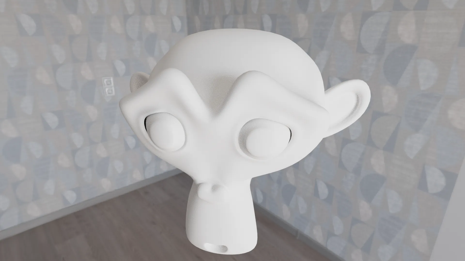
The cover image is rendered for 512 samples per pixel, 1280x720, and took about 2 minutes to render. It was tone-mapped in Blender's compositor.

For comparison, here's the exact same scene rendered with Blender Cycles at 32 samples, 1280x720, which took 11.46 seconds:

Why is my renderer worse?

Well I wrote mine in 2 weekends whereas Blender Cycles has been in development for years. But we can see that Cycles takes about 388 nanoseconds per pixel-sample, whereas my renderer only takes about 271 nanoseconds. This includes the amortized cost of the BVH construction and texture loading.

My render is faster per sample, but why is the image so much noisier at 16 times the number of samples?

The answer comes down to some interesting statistics. To get there, let's first cover what a ray tracer actually does.

The rendering equation

This is the rendering equation

For each pixel, we want to calculate \(L_o(\mathbf{x}, \omega_o)\), the radiance leaving the surface at \(\mathbf{x}\) in the direction \(\omega_o\). This is the sum of the emitted light \(L_e(\mathbf{x}, \omega_o)\) and the light reflected from all other directions.

Let's take a look at the second term:

This is an integral on the point of a surface over all directions where there could be incoming light. Ignoring transmission, this is the integral over the upper hemisphere, relative to the surface normal.

This consists of 3 terms:

\(f(\mathbf{x}, \omega_i, \omega_o)\) is the bidirectional reflectance distribution function (BRDF). Basically, it tells us how much light is reflected in direction \(\omega_o\) given that light is coming in from direction \(\omega_i\).

\(L_i(\mathbf{x}, \omega_i)\) is the incoming radiance from direction \(\omega_i\)

Finally, there's the cosine term \((\omega_i \cdot \mathbf{n})\). This exists because we do ray tracing from the camera to the light source, which is opposite to the direction that light travels. If we instead, for example, traced rays from the light source to the camera, this term would not be necessary.

This video explains this in more detail.

Estimating this integral

The second term, the integral is basically impossible to calculate analytically. This is because scenes are usually very complicated, consisting of many triangles, with BRDFs that could be defined by textures, and lights coming from many directions, or even from environment maps.

Instead, we use Monte Carlo integration. This is the principle of monte carlo integration:

To see how this works, let's consider the example of shading a pixel on a diffuse surface. The diffuse BSDF is literally just a constant: \(f(\mathbf{x}, \omega_i, \omega_o) = \text{albedo}\).

In my ray tracer, there's a struct Scene which implements the function sample(self, ray: &Ray) -> Color. This returns the radiance from the scene in the direction of ray. This translates to \(L_i(\mathbf{x}, \omega_i)\) in the rendering equation, where \(\mathbf{x}\) is the ray origin and \(\omega_i\) is the ray direction.

To compute this function, we cast a ray into the scene. This performs a ray-triangle intersection test against all the triangles in the scene (see the BVH section below). If the ray hits a triangle, the radiance is equal to \(L_o(\mathbf{x}, \omega_o)\), where \(\mathbf{x}\) is the point of intersection, and \(\omega_o\) is the direction of the ray pointing towards the camera.

\(\omega_o = -\omega_i = -\text{ray.direction}\).

To compute \(L_o\), we need to estimate the integral. To do that, we pick a random direction on the hemisphere. With this, we get a new \(\mathbf{x}\) and \(\omega_i\), with which we call \(L_i\) or sample again. We multiply this by the BRDF and the cosine term. This is a single sample (of which we did 512 in the cover image).

The problem with this approach

With the method I described, the outputs we get are very noisy (and actually slightly more so than the cover image).

We sample all directions with equal probability, even though all directions are not equally likely to contribute light. Due to this, the variance of this estimation is equal to the variance of the incoming light with respect to vectors on the hemisphere. If, say, all of the light is coming from the sun, which only takes up a very small portion of the hemisphere, the variance will be very high.

Additionally, there's the cosine term, which is 0 for directions that are perpendicular to the normal, and 1 for directions parallel.

Basically, we're wasting a lot of samples on directions that don't contribute much light.

Importance Sampling

Importance sampling is the idea of picking samples according to the distribution of light in the scene, in addition to the BRDF. Here's the equation

This video is really nice for learning the statistics behind importance sampling, and provides a very intuitive understanding of why it reduces variance (noise) of the estimate.

I want to preface that all of these methods are simply about sample efficiency. If you took an infinite number of samples, you'd get the exact same result with any method.

This is the only thing I implemented in my ray tracer. This picks directions according to the BRDF. For a diffuse surface, this is picking a cosine-weighted direction, i.e., zero probability of picking a direction perpendicular to the normal, and higher probability of picking directions parallel to the normal.

For mirror surfaces, this is picking a direction that's equal to the reflection of the incoming ray with respect to the normal: \(\omega_i = \text{reflect}(\omega_o, \mathbf{n})\).

Rewriting the rendering equation with this in mind:

The underscore signifies that we're picking values of \(\omega_i\) by using the BRDF as a probability distribution.

We also change the definition of f or the BRDF to include the cosine term here. I don't know if this is standard practice, but from what I can tell, it's not unsound.

There's still a problem, which is that we're not taking into account the distribution of light in the scene.

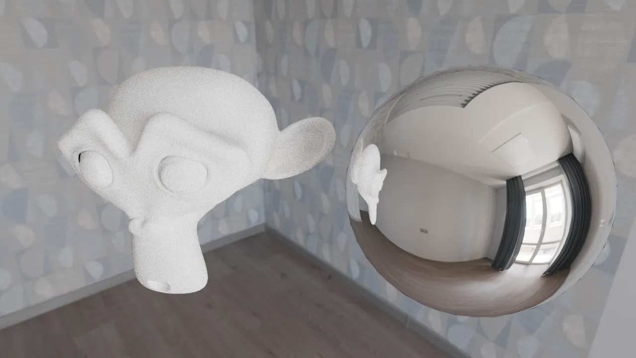
And to prove I'm doing this correctly, here's a scene with both a diffuse and a mirror surface:

Multiple Importance sampling

This is what Blender does, allowing it to render images with far less noise at lower sample counts. The idea is to pick a distribution \(p\) which takes into account not only the BRDF (\(f\)), but also the distribution of light in the scene. I don't know the math behind MIS or how it's implemented.

Colors

This is something I attempted to mess with myself, but realized that Rust community didn't have any OpenColorIO bindings and gave up. Instead, I just exported my renders as EXRs, and since the only texture I used was an environment map with linear Rec. 709 colors, linear assumptions in the renderer were sound, and I just used Blender's compositor to Filmic tone map the image and transform it to sRGB.

Ray triangle intersections

So at every computation of \(L_i\), we need to check if the ray intersects with any objects in the scene. If it doesn't, we simply return the environment map color.

To check whether or not it does, we would normally need to check intersection against every triangle in the scene. As you could guess, this becomes incredibly slow as the number of triangles increases.

To solve this, we use a BVH (Bounding Volume Hierarchy). This is a tree structure where each node contains a bounding box that contains all of the triangles in its children. This allows us to quickly discard large portions of the scene that the ray doesn't intersect with.

This video by Sebastian Lague is a great explanation and implementation of a BVH. I just used a crate that someone else made, which I regret in retrospect because it made it harder to do some performance optimizations.